Luis Felipe Luna-Reyes, Ph.D., Universidad de las Américas Puebla, Business School, This email address is being protected from spambots. You need JavaScript enabled to view it., Santa Catarina Mártr, Cholula, Mexico, 72810, Phone: +52 (222) 229-2060, Fax: +52 (222) 229-2062.
Jorge A. Durán-Encalada, Ph.D., Universidad de las Américas Puebla, Business School, This email address is being protected from spambots. You need JavaScript enabled to view it., Santa Catarina Mártr, Cholula, Mexico, 72810, Phone: +52 (222) 229-2060, Fax: +52 (222) 229-2062.
Eric R. Bandala, Ph.D., Universidad de las Américas Puebla, School of Engineering, This email address is being protected from spambots. You need JavaScript enabled to view it., Santa Catarina Mártr, Cholula, Mexico, 72810, Phone: +52 (222) 229-2031.
Abstract
This artcle presents a preliminary System Dynamics model developed to analyze the sustainability of a natural reserve in Mexico: the Tamiahua Wetlands. Wetlands are ofen referred to as nature’s kidneys because they flter contaminants from water. In spite of their importance, wetlands are endangered areas around the world. In order to build the model we take into account the Fishbanks model developed by Meadows (2004) as a startng point. Then, the model considers variables related to changes in total and economically actve populatons, and contaminants in water. The preliminary model presented in this study implies that fshing actvity in the Tamiahua Wetlands, together with contaminants from human actvity, have the potental to damage the diversity of species in the ecosystem, endangering its sustainability. Contnued work on the model is intended to explore appropriate ways of preserving Tamiahua, providing inhabitants with economic actvites that promote the sustainability of the region.
Keywords: sustainable development, Wetlands, Mexico, Tamiahua.
Introducton
This artcle introduces a preliminary System Dynamics model to analyze sustainability of a natural reserve located in the Northern bound of the State of Veracruz in Mexico: the Tamiahua Wetlands. The model presented in this study is the result of inital conversatons among researchers interested in regional development and the preservaton of the Tamiahua protected area, and builds upon such System Dynamics models as Fishbanks (Meadows, 2004). One of the authors of this inital study has been involved in extensive feld research in Tamiahua, collectng informaton about water quality. During his feldwork, he has observed a growth in the fshing industry followed by a decline on the actvity of fshing cooperatves. The reducton in fshing appears to be the result of a combinaton of such factors as increased fshing actvity, contaminaton and deterioraton of the diversity of species in the wetlands region.
The document is organized in fve more parts. The second secton consists of a literature review on the nature and characteristcs of wetlands, and the use of System Dynamics as a tool to study sustainability of fshing. The third secton describes the methods used in the study. The next two parts: Analysis and Results and Discussion, describe the model structure and some interestng behaviors of the model TAMIAHUA1, respectvely. Finally, the last secton offers some fnal remarks and suggestons for further work.
Literature review
Wetlands are ofen referred to as nature’s kidneys because they readily flter contaminants from water, there are also famous for their intrinsic beauty and importance as habitat for rare and endangered species as well as their role in carrying out basic ecological functons such as primary productvity, decompositon, nutrient cycling and regulaton of fluxes between land and water bodies. These ecosystems can also functon to remove and store nutrients and toxic pollutants in runoff from surrounding areas.
Partcularly, coastal wetlands play an important role in protectng coastal water quality. They are critcal ecosystems that help to regulate and maintain the hydrology by storing and releasing floodwaters. Wetlands are hard to defne mainly because they are transiton zones. Their hydrology is usually the most important factor determining its character. These regions are considered one of nature’s most efcient flters and usually are important nurseries for fsh, crabs, shellfsh, and an extensive variety of animals.
Despite their importance in the ecosystems, wetlands are endangered zones all around the world. Only in the USA, an annual loss of approximately 1.05 million hectares of wetlands is estmated (Josephson, 1992). Apart from agricultural conversion, wetlands are contnuously jeopardized as result of overfshing, burgeoning development, sediment contaminaton and nutrient polluton, all this is the result of growing populaton and increasing unplanned development in coastal countes. Such situaton in many cases promotes excessive exploitaton of fsheries and an increasing number of threatened, endangered and extnct indigenous species.
System Dynamics has been used in exploring the environmental management and sustainability in applicatons that tackle problems of forestry in Indonesia, irrigated lands in Spain, renewable resource management in Norway, wildlife management in the USA and blue-green algae bloom in the coastal waters of Australia (Cavana and Ford, 2004). What these applicatons have revealed is that modeling dynamically these complex problems with many factors can enlighten the implementaton of possible policies to alleviate the problem. System Dynamics has proven to be a useful tool when complex systems need to be re-oriented towards greater sustainability through policies that are quite different from those currently implemented and which should focus on the true driving factors of the system (Martnez Fernández and Esteve Selma, 2004). Our study subscribes to these assumptons and aims.
Partcularly, System Dynamics has been used successfully to analyze and study fshing systems in a variety of ways (Morecrof, 2007; Oto and Struben, 2004; Ruth, 1995). Most of these previous efforts were focused on analyzing the problem known as the “Tragedy of the Commons” and policies to control overexploitaton of fshing areas. The model presented in this artcle builds on previous work in System Dynamics and studies the impact of contaminants and of fshing actvites on the diversity of species in Tamiahua Wetlands.
Method
It is clear, from the analysis of the research site, that to achieve a sustainable and holistc understanding of the complexity faced by the Tamiahua Wetlands and its stakeholders, we need to go beyond simply predictng the fshing actvity. Economic and social variables interact dynamically with environmental and insttutonal variables.
To explore the effect of fshing on the interacton of other variables, a System Dynamics model was constructed. System Dynamics, originally known as Industrial Dynamics, is a creaton of Jay Forrester in the 1960s at the Massachusets Insttute of Technology (Forrester, 1961). System Dynamics is essentally a methodology which uses the theory of informaton feedback and control in order to evaluate organizatons and problems. The basic idea underpinning this approach is that any complex situaton can be described in terms of stocks and flows; flows being main actons increasing or decreasing the stocks. System Dynamics assumes that things are interconnected in complex closed paterns of causality, and that the world is made up of flows, stocks and feedback loops. Other assumptons include that informaton flows are intrinsically different from physical flows, and that non-linearites and tme-delays embedded in the system’s structure are important to understand the system behavior (Sterman, 2000). The main focus of the methodology is to capture the structure of complex problems, representng it in terms of stocks, flows and feedback loops, which consttutes a dynamic hypothesis to explain problematc behaviors. The model structure and behavior are then compared with known relatonships and behaviors in the system in several iteratons.
System Dynamics has been used in a variety of contexts, as a problem evaluaton on the premises that the structure of a system, that is the way the systems are connected, generates its behavior, aiming to predict the behavior of the system (Richardson and Pugh, 1989, Stave, 2003, Sterman, 2000). While statstcal forecastng models rely on equatons developed ex post, i.e. following observatons, System Dynamics aims frst to determine the systems structure consistng of positve and negatve relatonships between variables, feedback loops, systems archetypes, and delays (Sterman, 2000; Wolstenholme, 1982, 2003) followed by ex ante projecton where future system states are replicated from the System Dynamics model (Winz and Brierley, 2007).
As already mentoned in this artcle, the modeling effort is based upon the knowledge and experience of two experts, one on regional development, and the other on water and environment. Although obtaining quanttatve data to build the model has proven to be difcult, knowledge from feld work on the region has been used to ensure a beter understanding of behavior over tme and structural hypotheses. The model is stll in a preliminary stage, but inital model structure and some key parameters seem reasonable to expert judgment.
Analysis
The Tamiahua Wetlands
The Tamiahua Lagoon is located in the northern part of the state of Veracruz, Mexico. It is a coastal lagoon and covers an area of 217,500 acres, of 52.2 miles length, 9.6 miles width, and the depth of 2.2-3.3 yards. It has two water mouths, one in the north and another in the south, and is located in between two large rivers, Panuco in the north and Tuxpam in the south (see Figure 1).
There are some valuable natural resources in the area which comprise an important mangrove swamp towards the south of the lagoon and coral reef formatons to the east, on the Gulf of Mexico coast.
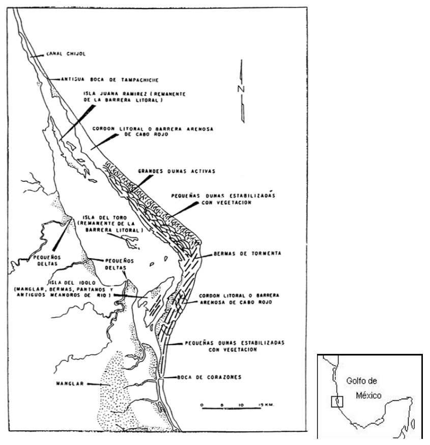
Source: Revista internacional de contaminación ambiental – Bioacumulación (2013).
The biodiversity of the place is rich, the area being inhabited by mollusk, crustacean, polychaeta, waterfowl, and a place for turtles laying eggs. Due to its ecology, botany, zoology, limnology, and hydrology richness, the Tamiahua was designated as a protected wetland included in the Ramsar Treaty of November 27th, 2005. The Ramsar Conventon provides the framework for natonal acton and internatonal cooperaton for the conservaton and wise use of wetlands and their resources.
However, in the last ten years, a polluton problem has been affectng fshing actvites in the lagoon. Industrial and residental pollutants are brought to the lagoon through 5 main rivers. The main types of pollutants are: hydrocarbon, agro-chemicals, fertlizers, metals and all sort of organic and solid waste (Albert, Bandala, Torres-Nacho, and Villanueva, 2006).
Socio-economic conditons
Surrounding the Tamiahua Lagoon there are 5 municipalites with a total populaton of 205,000 inhabitants. The economically actve populaton (EAP) amounts to 40 percent of total populaton (INEGI, 2005, 2010). The main economic actvity in this region is concentrated in the primary sector, mainly agriculture, as 75 per cent of the EAP is located in this sector. Only 2.5 percent operate in the manufacturing sector, and the rest of the EAP work in the service sector (INEGI, 2005, 2010). The net rate of populaton growth in the region is estmated at 1.8 percent annually.
The fshing actvity is carried out by approximately 4,000 people (Cooperatva Pesquera, Tamiahua, 2012). They are grouped in 340 business units known as fshing cooperatves, with an average size of 12 people. Out of 4,000 people, 60 percent, that is 2,400, are proprietors of the business units, and the remaining 1,600 fshermen work as employees. It is estmated that the total fleet is composed of 680 fshing boats, which means an average of 2 boats per company.
According to recent data, annual fsh catchment is about 12,750 tons. This amounts to an average catchment per boat of 18.75 tons per year, or 37.5 tons per company. The estmated price per ton in the intermediary market is US$1,500.
The market price of a boat is US$10,500, and it has a usable life of 20 years. The operatng cost for each boat is estmated to run at US$10,000 per year, including wages.
Cooperatves in Mexico, as the fshing ones in Tamiahua, normally receive fnancial support by the Federal Government. In partcular, the Ministry for Agricultural and Fishing Resources decides on fshing permits and funding for cooperatves afer an economic feasibility study.
Model descripton
The model TAMIAHUA1 consists of four main sectors and was built using Vensim PLE Version 5.8. The frst two sectors are similar to the ones used on the Fishbanks model (Meadows, 2004), and include the fsh populaton and the fleet size. The third sector includes populaton dynamics in the region, and the last sector considers the contaminaton level in the water of the wetlands.
Figure 2 shows the basic structure of fsh populaton and fshing. The red parts in the model are those that are unique to the model presented in this study. The stock of diversity of the species was important to include, given the key role that this diversity plays on the cleaning functon of wetlands and its impact on the growth of fsh populaton. As shown in the fgure, fshing practces in Tamiahua have been recognized to have an impact on the diversity of the species. Moreover, water contaminants and the diversity of the species have also had an impact on the populaton of fsh in the lagoon.
Figures 3 and 4 represent the growth of the fshing fleet. Figure 3 includes the representaton of the atractveness of the fshing industry compared to other actvites in the Tamiahua region. Proft is the difference between income and costs associated to fshing, and the proftability of other economic actvites was estmated using the minimum wage in Mexico. As shown in Figure 4, the funding to increase fleet size does not come in this region from profts in the fshing industry, but from subsidies provided by the State government. As described by one of the experts involved in the modeling process, fshing cooperatves’ need to increase the fleet or replace the existng boats exerts pressure on State government to provide more public funds to buy new boats.
Figure 5 shows the way in which the atractveness of the fshing industry atracts Tamiahua region inhabitants to join (or leave) fshing cooperatves.
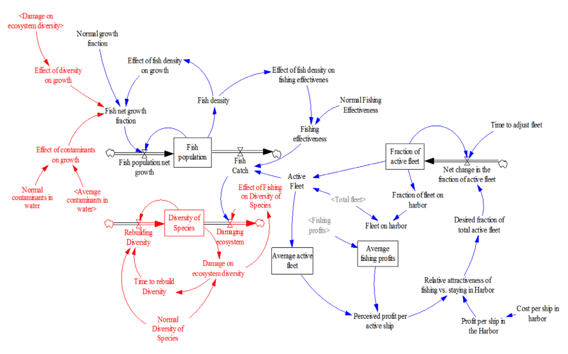
Source: Authors’ research on the basis of Meadows (2004).
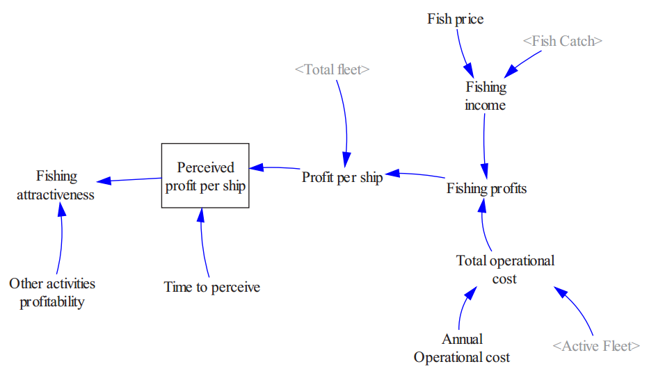
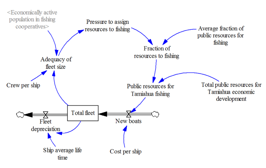
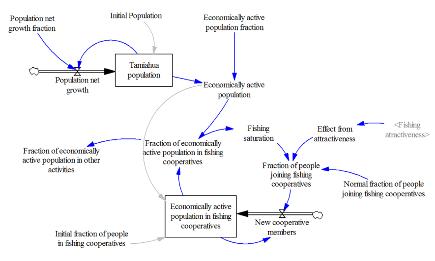
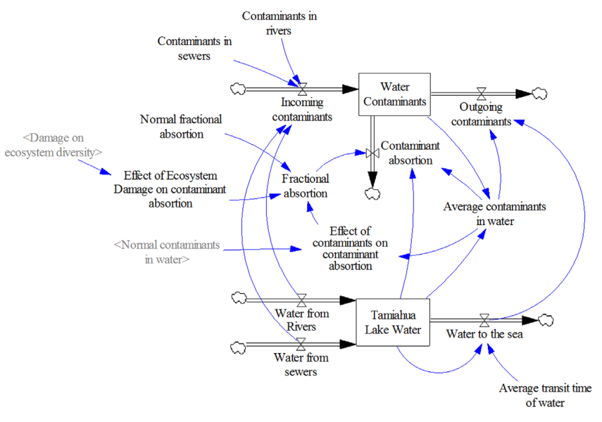
Finally, Figure 6 presents a theory of how contaminants come into the lagoon, and how the lagoon absorbs a fracton of these contaminants before the water reaches the sea. The Tamiahua lagoon has experienced a considerable increase on its polluton levels resultng from the release of chemicals produced in oil-related, industrial and agricultural actvites in the zone. During the last ffy years, the system has received oil spills from crude exploitaton facilites and oil pipelines. Besides, most of the municipalites setled in the surroundings of the lagoon lack sanitaton systems producing domestc wastewater and leachates from solid waste sites are released without any treatment to the lagoon (Albert et al., 2006). As shown in fgure 6, contaminants coming from industrial efuents upstream in the rivers and from sewers and human actvity may threaten the diversity of the species and have an impact on the absorpton capacity of the Tamiahua Lagoon.
Appendix A shows the parameters values and equatons that were used for the model.
Results and discussion
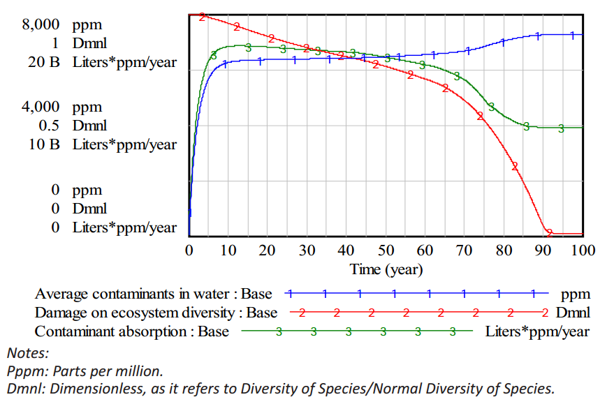
Figures 7, 8 and 9 show some of the behaviors of the model in a base scenario. Figure 7 shows the way in which fshing actvity slowly erodes the diversity of the species, eventually impairing the ability of the fsh populaton to reproduce in a healthy way. Figure 8 shows the dynamic behavior of the fleet size, the actve fleet and the fleet in harbor. As shown in the fgure, the impact on the fsh populaton promoted by contaminaton and the decrease on the diversity of the species is not yet enough in this model to have an impact on the fshing actvites. Given that the actual fleet size is similar to the simulated fleet size, this base scenario suggests that the observed decrease on fshing actvity in Tamiahua responds to the contaminaton of the wetlands or to the impact of the fshing techniques on the diversity of the species.
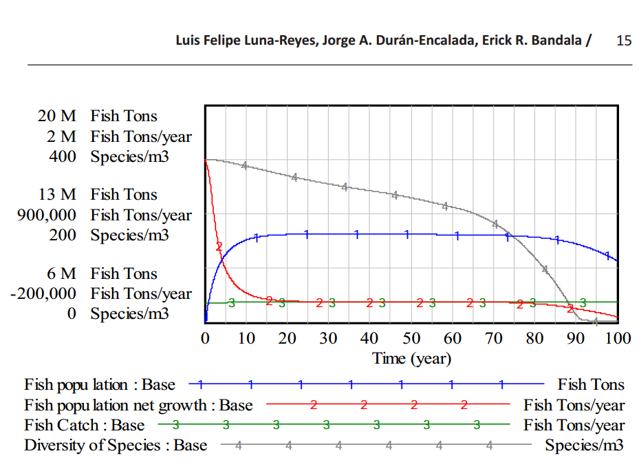
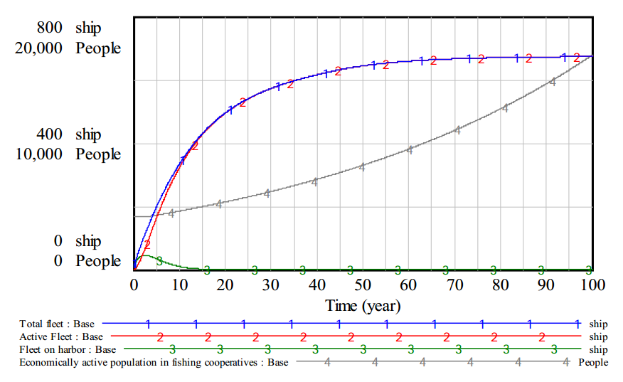
Figure 9 shows some key behaviors of the ecosystem. During the last years of the simulaton, it is possible to observe an important damage in the diversity of the species, which leads to an increase in contaminants in the lake, atributed mostly to the reducton in the capacity of the lagoon to absorb contaminants
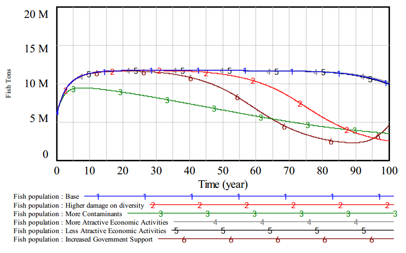
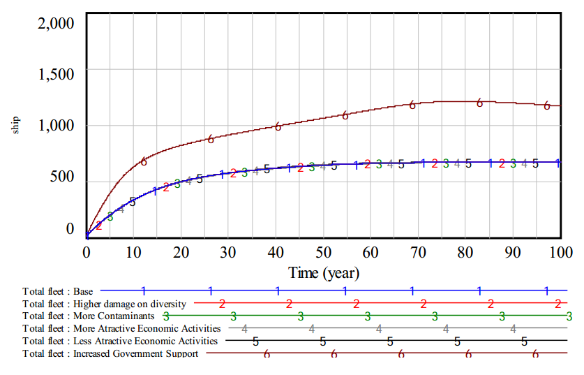
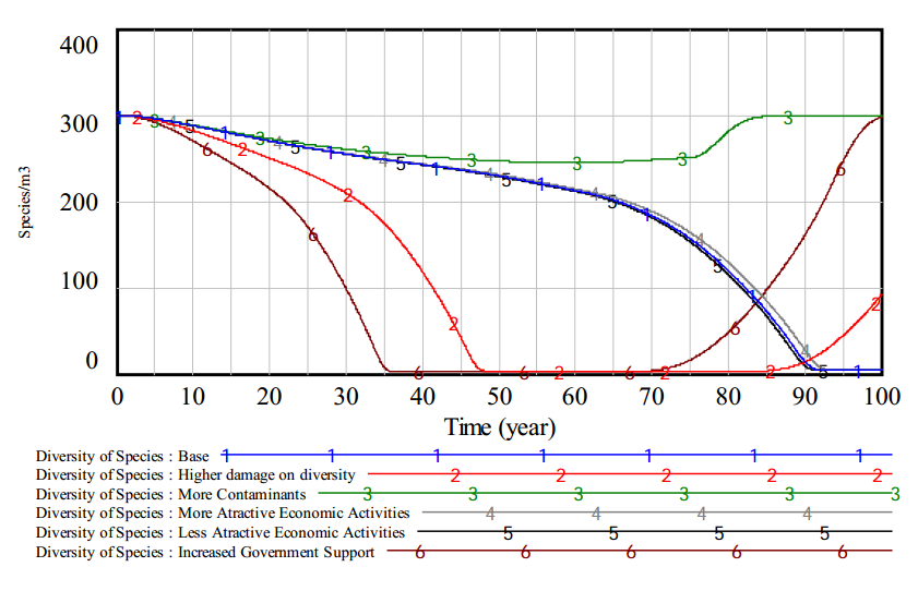
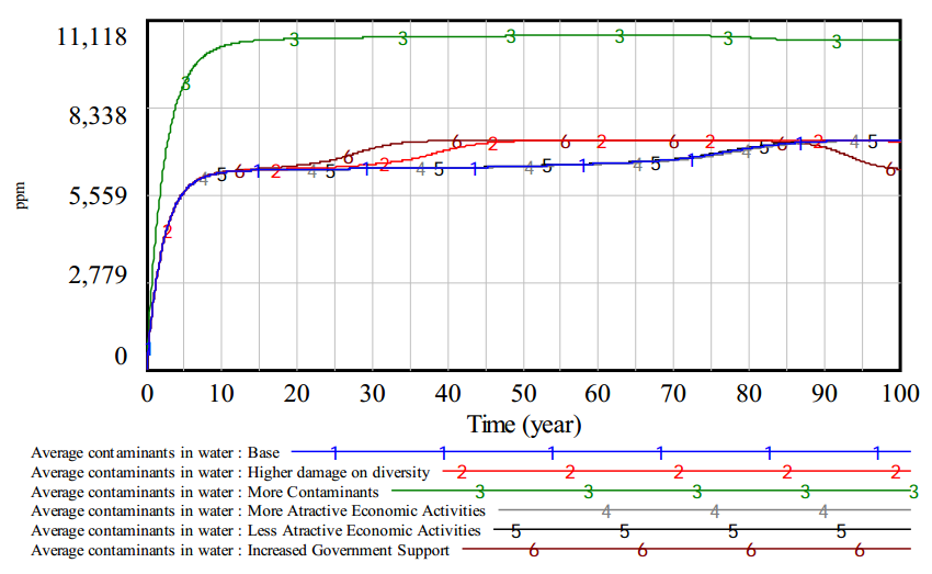
The inital exploratons with the model involved 5 parameter changes producing also 5 basic scenarios. In the frst scenario, we increased the damage on the ecosystem produced by the fshing actvity. The second scenario consists of an increase in incoming contaminants to the lagoon. The third and fourth scenarios involve changes in the atractveness of alternatve economic actvites, making fshing more or less atractve. The last scenario explores the impacts of increased resources from government to the fshing industry.
As shown in Figures 10 to 13, atractveness of alternatve economic actvites have a very limited impact on model behavior. The main reason is that the main source of economic resources to increase the fleet size is government funds. An increase in government funds, on the other hand, does have an impact on the sustainability of the ecosystem because it allows for the fleet size growth, acceleratng damage to the ecosystem, and collapse of the fshing industry. Increasing contaminants from rivers and changes in fshing practces for ones with higher environment impacts have an important impact on fsh populaton. Increased contaminants have a more contnuous impact, and increased impact from fshing practces contributes to a faster decline in fsh populaton.
Conclusion
In this short artcle, we presented a preliminary model to study the sustainability of the Tamiahua Lagoon considering the fshing actvity and the impact this actvity makes on the diversity of species in the lagoon. Additonally, the model includes the impact of contaminaton of the wetlands. Preliminary experiments suggest that fshing practces and contaminaton have the potental to create a signifcant imbalance in the system, apparently in a more important way that the actual fshing intensity.
Fishing actvity is considerably limited by the availability of government funds. In this way, government decisions on funding the fshing actvity affect the stability of the system.
Although the model presented in this study has a reasonable structure, it stll needs to be refned in terms of parameter values, mostly those associated to the ecosystem. We will contnue our experiments with the model to create a series of policy recommendatons to the State Government of Veracruz in Mexico.
References
- Albert, L., Bandala, E.R., Botello, A., Torres-Nachon, C., and Villanueva S. (2006). Toxic contaminants presence and its effects on health and environment at Tamiahua Lagoon, Veracruz. Consejo Estatal de Protección al Ambiente. Gobierno del Estado de Veracruz.
- Cavana, R.Y. and Ford, A. (2004). Environmental and resource system Editors’ introducton. System Dynamics Review, 20(2), 89–98.
- Cooperatva Pesquera Tamiahua (2012). Datos anuales de Cooperatva Pesquera de Tamiahua. Registros anuales.
- Forrester, J. (1961). Industrial Dynamics. Waltham, MIT, USA: Pegasus Communicatons.
- Insttuto Nacional de Estadístca Geografa e Información (2005). Censos Económicos 2004, INEGI: México.
- Insttuto Nacional de Estadístca Geografa e Información (2010). Censos Económicos 2009, INEGI: México.
- Insttuto Nacional de Estadístca Geografa e Información (2006). Populaton and Housing Countng 2005, INEGI: México.
- Insttuto Nacional de Estadístca Geografa e Información (2011). Populaton and Housing Countng 2010, INEGI: México.
- Josephson, J. (1992). Status of wetlands. Environmental Science and Technology 26(3): 422.
- Martnez Fernández, J. and Esteve Selma, M.A. (2004). The dynamics of water scarcity on irrigated landscapes: Mazarrón and Aguilas in south-eastern Spain. System Dynamics Review 20(2), 117–137.
- Meadows, D.L. (2004). FishBanks, Ltd. Durham, NH: Laboratory of Interactve Learning.
- Morecrof, J. (2007). Fish and ships – fshery dynamics with bounded ratonality. Paper presented at the 2007 Internatonal Conference of the System Dynamics Society, Boston, MA.
- Otto, P. and Struben, J. (2004). Gloucester fshery: Insights from a group modeling interventon. System Dynamics Review, 20(4), 287-312.
- Ruth, M. (1995). A system dynamics approach to modeling fsheries management issues: Implicatons for spatal dynamics and resoluton. System Dynamics Review, 11(3), 233-243.
- Stave, K.A. (2003). A systems dynamics model to facilitate public understanding of water management optons in Las Vegas, Nevada. Journal of Environmental Management, 67, 303-313.
- Richardson, G.P. and Pugh, A.L. (1989). Introducton to System Dynamics Modeling. Waltham MA: Pegasus Communicatons.
- Sterman, J. (2000). Business Dynamics, Systems Thinking and Modeling for a Complex World. USA: Irwin McGraw-Hill.
- Winz, I. and Brierley, G. (2007). The Use of System Dynamics Simulaton in Integrated Water Resources Management. Paper presented at the Systems Dynamics Conference 2007, University of Auckland, New Zealand.
- Wolstenholme, E.F. (1982). System Dynamics in Perspectve. The Journal of the Operatonal Research Society, 33(6), 547-556.
- Wolstenholme, E.F. (2003). Towards the defniton and use of a core set of archetypal structures in system dynamics. System Dynamics Review, 19(1), 7-26.
Electronic reference
- Revista internacional de contaminación ambiental - Bioacumulación (2013). Retrieved from:
https://www.google.com.mx/search?q=tamiahua+lagoon+mexico&source=lnms&tbm=isch&sa=X&ei=PEJXUuqgD66FyQGRnoHADw&ved=0CAcQ_AUoAQ&biw=1438&bih=655&dpr=1#facrc=_&imgdii=_&imgrc=Pq0Uon9RlCfAeM%3A%3B_jd1Dj7iSR_9xM%3Bhttp%253A%252F%252Fwww.scielo.org.mx%252Fimg%252Frevistas%252Frica%252Fv26n3%252Fa3f1.jpg%3Bhttp%253A%252F%252Fwww.scielo.org.mx%252Fscielo.php%253Fpid%253DS0188-49992010000300003%2526script%253Dsci_arttext%3B462%3B598
Appendix A. Parameters and model equations
| (001) | Active Fleet = Total fleet * Fraction of active fleet |
| Units: ship | |
| Number of ships fishing in the Wetlands | |
| (002) | Adequacy of fleet size = (Economically active population in fishing cooperatives / Crew per ship) / Total fleet |
| Units: Dmnl | |
| A ratio describing how well the current fleet employ people in Tamiahua. A ratio greater than reveals unemployed people | |
| (003) | Annual Operational cost = 245000 Units: pesos/(year*ship) |
| Cost of operating an active ship per year | |
| (004) | Average active fleet = SMOOTH ( Active Fleet, Time to register average) Units: ship |
| Average number of ships fishing in Tamiahua | |
| (005) | Average contaminants in water = Water Contaminants / Tamiahua Lake Water Units: ppm |
| Water contaminants measured in parts per million | |
| (006) | Average fishing profits = SMOOTH ( Fishing profits, Time to register average) Units: pesos/year |
| Average profits from fishing per year | |
| (007) | Average fraction of public resources for fishing = 0.1 Units: Dmnl |
| The average represents the importance to subsidize fishing by local government. | |
| (008) | Average transit time of water = 3 Units: year |
| This is the time that takes for water coming from rivers to reach the sea in its transit through the Wetlands | |
| (009) | Contaminant absorption = Average contaminants in water * Tamiahua Lake Water * Fractional absorption |
| Units: Liters*ppm/year | |
| This rate represents the cleaning process that happens in the Wetlands | |
| (010) | Contaminants in rivers = 5000 Units: ppm |
| These are contaminants coming from rivers, regularly they are fertilizers that accumulate in the river because of agricultural activities | |
| (011) | Contaminants in sewers = 12000 Units: ppm |
| These are contaminants coming from sewers, regularly these contaminants are city residuals that accumulate in the river because of urban activities, both residential and industrial | |
| (012) | Cost per ship = 250000 |
| Units: pesos/ship | |
| The cost of a ship in pesos | |
| (013) | Cost per ship in harbor = 50 Units: pesos/(year*ship) |
| The cost of having a ship in harbor per year | |
| (014) | Crew per ship = 6 Units: People/ship |
| The number of people needed to man a ship | |
| (015) | Damage constant = 0.0015 |
| Units: Species/(Fish Tons*m3) [0,1,0.001] | |
| A constant representing the damage on the diversity in species because of fishing. The diversity is important for the cleaning process that happens in the Wetlands | |
| (016) | Damage on ecosystem diversity = Diversity of Species / Normal Diversity of Species Units: Dmnl |
| This is the current status of the Wetlands relative to the normal count of species. | |
| (017) | Damaging ecosystem = Fish Catch * Effect of Fishing on Diversity of Species Units: Species/(year*m3) |
| This outflow represents erosion in the ecosystem as a result of fishing practices | |
| (018) | Desired fraction of total active fleet = DFTFC f ( “Relative attractiveness of fishing vs. staying in Harbor?) |
| Units: Dmnl | |
| This fraction determines the number of ships fishing as a result of the profitability of fishing | |
| (019) | DFTFC f ( [(-2,0)-(2,1)],(-2,1),(-1.6,0.98),(-1.2,0.9),(-0.8,0.8),(-0.4,0.66),(0,0.5),(0.4,0.34), (0.8,0.2),(1.2,0.1),(1.6,0.02),(2,0) ) |
| Units: Dmnl | |
| This is the function of the fraction of ships fishing. The more profitable the fishing is, the more ships do it. | |
| (020) | Diversity of Species = INTEG( Rebuilding Diversity - Damaging ecosystem, Normal Diversity of Species ) |
| Units: Species/m3 | |
| A level representing current bio-diversity in Tamiahua wetlands. | |
| (021) | ECCA f ( [(0,0.5)-(2,1.5)],(0,1.2),(0.2,1.19737),(0.4,1.18421),(0.6,1.15789),(0.8,1.09649), (1,1),(1.2,0.864035),(1.4,0.710526),(1.6,0.600877),(1.8,0.530702),(2,0.5) ) |
| Units: Dmnl | |
| This function describes the ability of the Wetlands to clean themselves under different concentrations of contaminants. | |
| (022) | ECFNG f ( [(0,-1)-(2,1)],(0,1),(0.2,0.903509),(0.4,0.719298),(0.6,0.5),(0.8,0.27193), (1,0),(1.2,-0.192982),(1.4,-0.307018),(1.6,-0.385965),(1.8,-0.45614),(2,-0.5) ) Units: Dmnl |
| This function describes the impacts of water contamination on the ability of the fish population to reproduce | |
| (023) | Economically active population = Economically active population fraction* Tamiahua population |
| Units: People | |
| People in working age available to work outside home | |
| (024) | Economically active population fraction = 0.3 Units: Dmnl |
| Fraction of people in working age available to work outside home | |
| (025) | Economically active population in fishing cooperatives = INTEG( New cooperative members, Initial fraction of people in fishing cooperatives * Economically active population) Units: People |
| People working in coop fisheries | |
| (026) | EDCFG f ( [(0,-4)-(2,2)],(0,0.8),(0.2,1.07895),(0.4,1.26316),(0.6,1.21053),(0.8,0.921053), (1,0.394737),(1.19878,-0.0526316),(1.38226,-0.473684),(1.57187,-1.02632), |
| (1.78593,-1.5),(2,-2.13158) ) Units: Dmnl | |
| This function represents the ability of the fish population to reproduce, given a certain fish density | |
| (027) | EDG f ( [(0,-1)-(1,1)],(0,-0.5),(0.1,-0.464912),(0.2,-0.403509),(0.3,-0.289474), (0.4,-0.149123),(0.5,0),(0.6,0.22807),(0.7,0.491228),(0.8,0.754386),(0.9,0.903509),(1,1) ) Units: Dmnl |
| This function describes the impacts of bio-diversity on the ability of the fish population to reproduce | |
| (028) | EEDCA f ( [(0,0)-(1,1)],(0,0.5),(0.1,0.504386),(0.2,0.508772),(0.3,0.530702), (0.4,0.570175),(0.5,0.635965),(0.6,0.763158),(0.7,0.855263),(0.8,0.938596),(0.9,0.973684), (1,1) ) |
| Units: Dmnl | |
| This function describes the impacts of bio-diversity on the ability of the Wetlands to clean themselves | |
| (029) | EFA f ( [(0,-1)-(2,1.2)],(0,-0.5),(0.2,-0.150877),(0.4,0.157895),(0.6,0.466667),(0.8,0.727193), (1,1),(1.2,1.13246),(1.4,1.1807),(1.6,1.1807),(1.8,1.1807),(2,1.2) ) |
| Units: Dmnl | |
| This function describes the impacts of fishing attractiveness on the number of people that wants to work on this industry | |
| (030) | EFDS f ( [(0,0)-(1,1.2)],(0,0),(0.025,0.6),(0.05,0.8),(0.075,0.95),(0.1,0.99),(0.2,1),(0.3,1), (0.4,1),(0.5,1),(0.6,1),(0.7,1),(0.8,1),(0.9,1),(1,1) ) |
| Units: Dmnl | |
| This function describes the effect of fishing practices on bio-diversity | |
| (031) | Effect from attractiveness = EFA f ( Fishing attractiveness ) Units: Dmnl |
| The fishing attractiveness function | |
| (032) | Effect of contaminants on contaminant absorption = ECCA f ( Average contaminants in water / Normal contaminants in water ) |
| Units: Dmnl | |
| The effect of contaminants on contaminant absorption | |
| (033) | Effect of contaminants on growth = ECFNG f ( Average contaminants in water / Normal contaminants in water ) |
| Units: Dmnl | |
| The impact of contamination on the fish population ability to regenerate | |
| (034) | Effect of diversity on growth = EDG f ( Damage on ecosystem diversity) Units: Dmnl |
| The effect of bio-diversity on the fish population ability to reproduce | |
| (035) | Effect of Ecosystem Damage on contaminant absorption = EEDCA f ( Damage on ecosystem diversity) |
| Units: Dmnl | |
| The impact of bio-diversity on the ability of the Wetlands of cleaning themselves | |
| (036) | Effect of fish density on fishing effectiveness = SEDC f ( Fish density) Units: Dmnl |
| The impact of fish density on fishing | |
| (037) | Effect of fish density on growth = EDCFG f ( Fish density ) Units: Dmnl |
| The impact of fish density on fish population net growth | |
| (038) | Effect of Fishing on Diversity of Species = Damage constant * EFDS f ( Damage on ecosystem diversity ) |
| Units: Species/(Fish Tons*m3) | |
| The impact of fishing on the wetlands bio-diversity | |
| (039) | FINAL TIME = 100 |
| Units: year | |
| The final time for the simulation. | |
| (040) | Fish Catch = Active Fleet * Fishing effectiveness Units: Fish Tons/year |
| This rate describes the yearly catch | |
| (041) | Fish density = Fish population / Tamiahua lake carrying capacity Units: Dmnl |
| A ratio describing how much fish are in the Wetlands compared to the total capacity | |
| (042) | Fish net growth fraction = Effect of fish density on growth * Effect of contaminants on growth* Effect of diversity on growth * Normal growth fraction |
| Units: 1/year | |
| This is the yearly growth fraction considering all factors that have an impact on it | |
| (043) | Fish population = INTEG( Fish population net growth - Fish Catch, 6e+006) Units: Fish Tons |
| Fish population in the Tamiahua wetlands | |
| (044) | Fish population net growth = Fish population * Fish net growth fraction Units: Fish Tons/year |
| The Fish population net growth rate | |
| (045) | Fish price = 15000 Units: pesos/Fish Tons Price per fish ton |
| (046) | Fishing attractiveness = Perceived profit per ship / Other activities profitability Units: Dmnl |
| A ratio comparing fishing profitability to the profitability of other economic activities | |
| (047) | Fishing effectiveness = Normal Fishing Effectiveness * Effect of fish density on fishing effectiveness |
| Units: Fish Tons/(year*ship) | |
| The effectiveness of every ship in catching fish, as a function of fish density | |
| (048) | Fishing income = Fish Catch * Fish price Units: pesos/year |
| Total income from fishing | |
| (049) | Fishing profits = Fishing income - Total operational cost Units: pesos/year |
| Net profit from fishing | |
| (050) | Fishing saturation = FS f ( Fraction of economically active population in fishing cooperatives) Units: Dmnl |
| The current limits of job supply in the fishing industry | |
| (051) | Fleet depreciation = Total fleet / Ship average life time Units: ship/year |
| Fleet depreciates linearly on a given average life time | |
| (052) | Fleet on harbor = Total fleet * Fraction of fleet on harbor Units: ship |
| Number of ships that are left on the harbor instead of going fishing | |
| (053) | Fraction of active fleet = INTEG( Net change in the fraction of active fleet, 0.05) Units: Dmnl |
| The fraction of ships that are actually fishing | |
| (054) | Fraction of economically active population in fishing cooperatives = Economically active population in fishing cooperatives / Economically active population |
| Units: Dmnl | |
| The fraction of people working in fishing cooperatives | |
| (055) | Fraction of economically active population in other activities = 1 - Fraction of economically active population in fishing cooperatives |
| Units: Dmnl | |
| The fraction of people working in other industries different from fishing | |
| (056) | Fraction of fleet on harbor = 1 - Fraction of active fleet Units: Dmnl |
| This is the fraction of the fleet that cooperatives decide to keep on the harbor | |
| (057) | Fraction of people joining fishing cooperatives = Effect from attractiveness * Fishing saturation * Normal fraction of people joining fishing cooperatives |
| Units: 1/year | |
| The fraction of people joining the fishing industry because of the attractiveness of the industry, as well as the demand for crew members | |
| (058) | Fraction of resources to fishing = Average fraction of public resources for fishing * Pressure to assign resources to fishing |
| Units: Dmnl | |
| The actual amount of public money to invest in fishing cooperatives | |
| (059) | Fractional absorption = Effect of contaminants on contaminant absorption * Effect of Ecosystem Damage on contaminant absorption * Normal fractional absorption Units: 1/year |
| The fraction of contaminants that the Wetlands can manage per year | |
| (060) | FS f ( [(0,0)-(1,1.3)],(0,1.2),(0.1,1.2),(0.2,1.2),(0.3,1.19167),(0.4,1.15746),(0.5,1.11184), (0.6,1.04912),(0.7,0.992105),(0.8,0.87807),(0.9,0.615789),(1,0) ) |
| Units: Dmnl | |
| The function of job supply saturation in the fishing industry | |
| (061) | Incoming contaminants = Contaminants in rivers * Water from Rivers + Contaminants in sewers * Water from sewers |
| Units: Liters*ppm/year | |
| Total contaminants incoming into the Wetlands | |
| (062) | Initial fraction of people in fishing cooperatives = 0.07 Units: Dmnl |
| Model assumption about the initial value of the fraction of people working in the fishing industry | |
| (063) | Initial Population = 200000 Units: People |
| Model assumption about initial values of the population in the region | |
| (064) | INITIAL TIME = 0 Units: year |
| The initial time for the simulation. | |
| (065) | Net change in the fraction of active fleet = ( Desired fraction of total active fleet - Fraction of active fleet ) / Time to adjust fleet |
| Units: 1/year | |
| The rate adjusting the fraction of fleet fishing per year | |
| (066) | New boats = Public resources for the Tamiahua fishing / Cost per ship Units: ship/year |
| Ship construction rate, assuming that all ship construction is subsidized by government | |
| (067) | New cooperative members = Fraction of people joining fishing cooperatives * Economically active population in fishing cooperatives |
| Units: People/year | |
| The rate of new workers joining the fishing industry | |
| (068) | Normal contaminants in water = 10000 Units: ppm |
| Reference value for contaminants in the Wetlands | |
| (069) | Normal Diversity of Species = 300 Units: Species/m3 |
| Reference value for diversity in the Wetlands | |
| (070) | Normal Fishing Effectiveness = 20 Units: Fish Tons/(year*ship) Average fishing capacity per boat |
| (071) | Normal fraction of people joining fishing cooperatives = 0.01 Units: 1/year |
| Average growth of workforce in the fishing industry | |
| (072) | Normal fractional absorption = 0.1 Units: 1/year |
| Average absorption of contaminants | |
| (073) | Normal growth fraction = 0.2 Units: 1/year |
| Average fertility of the fish population per year | |
| (074) | Other activities profitability = 20000 Units: pesos/(year*ship) |
| Average profit in other industries competing with the fishing industry | |
| (075) | Outgoing contaminants = Water to the sea * Average contaminants in water Units: Liters*ppm/year |
| Contaminants that leave the Wetlands into the sea | |
| (076) | PARF f ( [(0,0)-(2,2)],(0,0),(0.2,0.105263),(0.4,0.298246),(0.6,0.517544),(0.8,0.77193), (1,1),(1.2,1.2193),(1.4,1.37719),(1.6,1.4386),(1.8,1.45614),(2,1.5) ) |
| Units: Dmnl | |
| The function describing the effect of the adequacy of the fleet size into the pressure to build more ships by government | |
| (077) | Perceived profit per active ship = Average fishing profits / Average active fleet Units: pesos/(year*ship) |
| The perception of profit of ships fishing that will have an impact on the fraction of active | |
| boats | |
| (078) | Perceived profit per ship = SMOOTH ( Profit per ship, Time to perceive) Units: pesos/(year*ship) |
| Perception of ship profitability. Which will have an impact on working in the fishing industry | |
| (079) | Population net growth = Population net growth fraction * Tamiahua population Units: People/year |
| Net rate of population growth | |
| (080) | Population net growth fraction = 0.015 Units: 1/year |
| Average population growth | |
| (081) | Pressure to assign resources to fishing = PARF f ( Adequacy of fleet size) Units: Dmnl |
| A function of the adequacy of job supply in the fishing industry | |
| (082) | Profit per ship = Fishing profits / Total fleet Units: pesos/(year*ship) |
| (083) | Profit per ship in the Harbor = 0 - Cost per ship in harbor Units: pesos/(year*ship) |
| A reference value to decide on sending ships to fish | |
| (084) | Public resources for Tamiahua fishing = Fraction of resources to fishing * Total public resources for Tamiahua economic development |
| Units: pesos/year | |
| Amount of public money used to increase the fleet | |
| (085) | Rebuilding Diversity = ( Normal Diversity of Species - Diversity of Species) / Time to rebuild Diversity |
| Units: Species/(year*m3) | |
| Regeneration of the Wetlands ecosystem | |
| (086) | “Relative attractiveness of fishing vs. staying in Harbor? = Perceived profit per active ship / Profit per ship in the Harbor |
| Units: Dmnl | |
| A ration comparing active boats profit to costs of staying idle | |
| (087) | SAVEPER = TIME STEP |
| Units: year | |
| The frequency with which output is stored. | |
| (088) | SEDC f ( [(0,0)-(2,1.5)],(0,0),(0.149847,0.447368),(0.388379,0.754386),(0.599388,0.912281), (0.798165,0.960526),(1,1),(1.19878,1.03947),(1.41896,1.08553),(1.59633,1.16447),(1.8,1.2), (2,1.2) ) |
| Units: Dmnl | |
| The relationship between fish density and ship effectiveness | |
| (089) | Ship average life time = 15 Units: year |
| Working life of a boat | |
| (090) | Tamiahua lake carrying capacity = 1e+007 Units: Fish Tons |
| Estimated max fish population | |
| (091) | Tamiahua Lake Water = INTEG (Water from Rivers + Water from sewers - Water to the sea, 2.4e+007) |
| Units: Liters | |
| Total water in the wetlands | |
| (092) | Tamiahua population = INTEG( Population net growth, Initial Population) Units: People |
| Total population | |
| (093) | TIME STEP = 0.0625 Units: year |
| The time step for the simulation. | |
| (094) | Time to adjust fleet = 3 Units: year |
| Average time to make changes on the fraction of active fleet | |
| (095) | Time to perceive = 2 Units: year |
| Average time to perceive fishing industry profitability | |
| (096) | Time to rebuild Diversity = WITH LOOKUP( Damage on ecosystem diversity, ([(0,0)-(1,50)], (0,50),(0.1,34.6491),(0.2,25.4386),(0.3,18.6404),(0.4,14.693),(0.5,10.7456),(0.6,7.45614), (0.7,4.82456),(0.8,3.28947),(0.9,2.19298),(1,1) ) ) |
| Units: year | |
| A function describing the effect of ecosystem damage on the ability of the wetlands to regenerate | |
| (097) | Time to register average = 1 Units: year |
| Average reporting time in the fishing industry | |
| (098) | Total fleet = INTEG( New boats - Fleet depreciation, 10) Units: ship |
| (099) | Total operational cost = Annual Operational cost * Active Fleet Units: pesos/year |
| Total cost of active fleet | |
| (100) | Total public resources for Tamiahua economic development = 7.5e+007 Units: pesos/year |
| Public resources available | |
| (101) | Water Contaminants = INTEG( Incoming contaminants - Contaminant absorption - Outgoing contaminants, 1e+009) |
| Units: Liters*ppm | |
| Total contaminants on the wetlands | |
| (102) | Water from Rivers = 4e+006 Units: Liters/year |
| Water incoming from rivers | |
| (103) | Water from sewers = 4e+006 Units: Liters/year |
| Water incoming from sewers | |
| (104) | Water to the sea = Tamiahua Lake Water / Average transit time of water Units: Liters/year |
| Water flowing to the sea |

